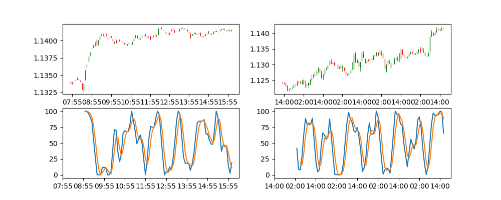
この記事では、1分足から5分足と1時間足のローソク足チャートを作成し、
その下にそれぞれのDTオシレーターを表示するスクリプトを作成します。
1分足の取得
今後GymのEnvに使っていきたいので、足を取得する部分は以前作ったEnvをそのまま使用します。
余計なことも書いてあるので適宜無視してください。
ただし、EnvではdropしていたOpenの値は必要になるので残すように変更しておきます。
ローソク足の作成、表示
mpl_financeを使用してローソク足チャートを表示します。
ポイント
xticksに日付時刻をそのまま使用してしまうと休日などで時刻のギャップが空いた際にチャートも空白になってしまうので、
xtickにはダミーの連番を用います。
dummy_indices_5m = np.linspace(0, len(target_5m), len(target_5m))
そして、xticklabelsに日付時刻を使用することで表示上は日付時刻が表示されます。
# DTOは1つ減るのでtickを合わせるため1始まり
x_tick = [i for i in np.array(indices_5m.to_pydatetime())][1::12]
x_tick_labels_5m = [i.strftime('%H:%M') for i in x_tick]
ax.set(xticks=dummy_indices_5m[1::12], xticklabels=x_tick_labels_5m)
DTOの作成、表示
DTOを作成します。
今回のパラメータは
period_rsi = 8
period_stoch = 5
period_sk = 3
period_sd = 3
で作成します。
RSIの計算
RSIの計算方法は色々なサイトに載っているのでそれを参考にしてください。
$$ \rm{RSI} = 100 – \frac{100}{1 + \rm{RS}} $$
# RSI計算(8)
close = target_5m['close']
diff = close.diff()[1:]
up, down = diff.copy(), diff.copy()
up[up < 0] = 0
down[down > 0] = 0
up_sma = up.rolling(window=8, center=False).mean()
down_sma = down.abs().rolling(window=8, center=False).mean()
rs = up_sma / down_sma
rsi = 100.0 - (100.0 / (1.0 + rs))
DTOの計算
DTOはストキャスティクスRSIを平滑化させたものなので、そのように作成します。
(参考:DT オシレーターのソースを読み解く)
# DTOの計算
rolling = rsi.rolling(period_stoch)
llv = rolling.min()
hhv = rolling.max()
sto_rsi = 100 * ((rsi - llv) / (hhv - llv))
sk = sto_rsi.rolling(period_sk).mean()
sd = sk.rolling(period_sd).mean()
結果
ソース全文
from random import random

import numpy as np
import os

from builtins import range, print
from builtins import Exception

import datetime

import pandas
from dateutil import relativedelta
import matplotlib.pyplot as plt
import mpl_finance as mpf


class FxDtoEnv:
    def __init__(self):
        # 観測できる足数
        self.visible_bar = 100
        # CSVファイルのパス配列(最低4ヶ月分を昇順で)
        self.csv_file_paths = []
        now = datetime.datetime.now()
        for _ in range(4):
            now = now - relativedelta.relativedelta(months=1)
            filename = 'DAT_MT_EURUSD_M1_{}.csv'.format(now.strftime('%Y%m'))
            if not os.path.exists(filename):
                print('ヒストリーファイルが存在していません。下記からダウンロードしてください。', filename)
                print('http://www.histdata.com/download-free-forex-historical-data/?/metatrader/1-minute-bar-quotes/EURUSD/')
                raise Exception('ヒストリーファイルが存在していません。')
            else:
                self.csv_file_paths.append(filename)

        self.data = pandas.DataFrame()
        for path in self.csv_file_paths:
            csv = pandas.read_csv(path,
                                  names=['date', 'time', 'open', 'high', 'low', 'close', 'v'],
                                  parse_dates={'datetime': ['date', 'time']},
                                  dtype={'datetime': np.long, 'open': np.float32, 'high': np.float32, 'low': np.float32, 'close': np.float32}
                                  )
            csv.index = csv['datetime']
            csv['datetime'] = csv['datetime'].astype(np.long)
            # ohlcを作る際には必要
            # csv = csv.drop('datetime', axis=1)
            # csv = csv.drop('open', axis=1)
            # histdata.comはvolumeデータが0なのでdrop
            csv = csv.drop('v', axis=1)
            self.data = self.data.append(csv)
            # 最後に読んだCSVのインデックスを開始インデックスとする
            self.read_index = len(self.data) - len(csv)

        self.read_index = int(random() * len(self.data))
        self.tickets = []

    def make_obs(self, mode):
        """
        5分足、1時間足の2時系列データをvisible_bar本分作成する
        :return:
        """
        target = self.data.iloc[self.read_index - 60 * env.visible_bar: self.read_index]
        if mode == 'human':
            m5 = np.array(target.resample('5min').agg({'high': 'max',
                                                          'low': 'min',
                                                          'close': 'last'}).dropna().iloc[-1 * self.visible_bar:][target.columns])
            h1 = np.array(target.resample('1H').agg({'high': 'max',
                                                        'low': 'min',
                                                        'close': 'last'}).dropna().iloc[-1 * self.visible_bar:][target.columns])
            return np.array([m5, h1])
        elif mode == 'ohlc_array':
            m5 = np.array(target.resample('5min').agg({'high': 'max',
                                                          'low': 'min',
                                                          'close': 'last'}).dropna().iloc[-1 * self.visible_bar:][target.columns])
            h1 = np.array(target.resample('1H').agg({'high': 'max',
                                                        'low': 'min',
                                                        'close': 'last'}).dropna().iloc[-1 * self.visible_bar:][target.columns])
            return np.array([m5, h1])


period_rsi = 8
period_stoch = 5
period_sk = 3
period_sd = 3

env = FxDtoEnv()

target = env.data.iloc[env.read_index - 60 * env.visible_bar: env.read_index]

# humanの場合はmatplotlibでチャートのimgを作成する?
fig = plt.figure(figsize=(10, 4))
# ローソク足は全横幅の太さが1である。表示する足数で割ってさらにその1/3の太さにする
width = 1.0 / env.visible_bar / 3
# 5分足
ax = plt.subplot(2, 2, 1)
# y軸のオフセット表示を無効にする。
ax.get_yaxis().get_major_formatter().set_useOffset(False)
target_5m = target['close'].resample('5min').ohlc().dropna().iloc[-1 * env.visible_bar:]
indices_5m = target_5m.index
dummy_indices_5m = np.linspace(0, len(target_5m), len(target_5m))
data_5m = pandas.DataFrame({'datetime': dummy_indices_5m,
                        'open': target_5m['open'],
                         'high': target_5m['high'],
                         'low': target_5m['low'],
                         'close': target_5m['close']}).values
mpf.candlestick_ohlc(ax, data_5m, width=width, colorup='g', colordown='r')

# DTOは1つ減るのでtickを合わせるため1始まり
x_tick = [i for i in np.array(indices_5m.to_pydatetime())][1::12]
x_tick_labels_5m = [i.strftime('%H:%M') for i in x_tick]
ax.set(xticks=dummy_indices_5m[1::12], xticklabels=x_tick_labels_5m)

# DTO(8,5,3,3)
ax = plt.subplot(2, 2, 3)
# RSI計算(8)
close = target_5m['close']
diff = close.diff()[1:]
up, down = diff.copy(), diff.copy()
up[up < 0] = 0
down[down > 0] = 0
up_sma = up.rolling(window=8, center=False).mean()
down_sma = down.abs().rolling(window=8, center=False).mean()
rs = up_sma / down_sma
rsi = 100.0 - (100.0 / (1.0 + rs))

# DTOの計算
rolling = rsi.rolling(period_stoch)
llv = rolling.min()
hhv = rolling.max()
sto_rsi = 100 * ((rsi - llv) / (hhv - llv))
sk = sto_rsi.rolling(period_sk).mean()
sd = sk.rolling(period_sd).mean()

dto_indices_5m = sk.index
dummy_indices_dto_5m = np.linspace(0, len(dto_indices_5m), len(dto_indices_5m))
ax.plot(dummy_indices_dto_5m, sk, label="sk")
ax.plot(dummy_indices_dto_5m, sd, label="sd")

x_tick = [i for i in np.array(dto_indices_5m.to_pydatetime())][::12]
x_tick_labels_dto_5m = [i.strftime('%H:%M') for i in x_tick]
ax.set(xticks=dummy_indices_dto_5m[::12], xticklabels=x_tick_labels_dto_5m)

# 1時間足
ax = plt.subplot(2, 2, 2)
# y軸のオフセット表示を無効にする。
ax.get_yaxis().get_major_formatter().set_useOffset(False)
target_1h = target['close'].resample('1H').ohlc().dropna().iloc[-1 * env.visible_bar:]
indices_1h = target_1h.index
dummy_indices_1h = np.linspace(0, len(target_1h), len(target_1h))
data_1h = pandas.DataFrame({'datetime': dummy_indices_1h,
                            'open': target_1h['open'],
                            'high': target_1h['high'],
                            'low': target_1h['low'],
                            'close': target_1h['close']}).values
mpf.candlestick_ohlc(ax, data_1h, width=width, colorup='g', colordown='r')

# DTOは1つ減るのでtickを合わせるため1始まり
x_tick = [i for i in np.array(indices_1h.to_pydatetime())][1::12]
x_tick_labels_1h = [i.strftime('%H:%M') for i in x_tick]
ax.set(xticks=dummy_indices_1h[1::12], xticklabels=x_tick_labels_1h)

# DTO(8,5,3,3)
ax = plt.subplot(2, 2, 4)
# RSI計算(8)
close = target_1h['close']
diff = close.diff()[1:]
up, down = diff.copy(), diff.copy()
up[up < 0] = 0
down[down > 0] = 0
up_sma = up.rolling(window=8, center=False).mean()
down_sma = down.abs().rolling(window=8, center=False).mean()
rs = up_sma / down_sma
rsi = 100.0 - (100.0 / (1.0 + rs))

# DTOの計算
rolling = rsi.rolling(period_stoch)
llv = rolling.min()
hhv = rolling.max()
sto_rsi = 100 * ((rsi - llv) / (hhv - llv))
sk = sto_rsi.rolling(period_sk).mean()
sd = sk.rolling(period_sd).mean()

dto_indices_1h = sk.index
dummy_indices_dto_1h = np.linspace(0, len(dto_indices_1h), len(dto_indices_1h))
ax.plot(dummy_indices_dto_1h, sk, label="sk")
ax.plot(dummy_indices_dto_1h, sd, label="sd")

x_tick = [i for i in np.array(dto_indices_1h.to_pydatetime())][::12]
x_tick_labels_dto_1h = [i.strftime('%H:%M') for i in x_tick]
ax.set(xticks=dummy_indices_dto_1h[::12], xticklabels=x_tick_labels_dto_1h)

plt.show()


コメント