最近Python機械学習を読み進めているのですが、その学習メモです。
パーセプトロン
用語
- 入力値:\( x \)
- 重みベクトル:\( w \)
- 総入力:\( z = w_1x_1 + … + w_mx_m = w^Tx \)
- しきい値:\( \theta \)
- 活性化関数(単位ステップ関数、ヘビサイド関数):\( \phi \)
(mathjaxのせいで数式が表示されない)
$$ \phi = \begin{eqnarray}\left{\begin{array{l}1(z\geq\theta) \-1(z<\theta)\end{array}\right.\end{eqnarray} $$ -
学習率:\( \eta \)
パーセプトロンの学習規則
- 重みを0または値の小さい乱数で初期化
- トレーニングサンプル\( x^{(i)} \)ごとに以下の手順を実行
- 出力値\( \hat{y} \)を計算する
- 重みを更新する
各重み\( w_j \)の更新法
$$ w_j := w_j + \Delta w_j $$
\( \Delta w_j \)の算出
$$ \Delta w_j = \eta(y^{(i)} – \hat{y}^{(i)})x_j^{(i)} $$
\( y^{(i)} \):本当のクラスラベル
\( \hat{y}^{(i)} \):予測されたクラスラベル
予測が当たった場合
重みは更新されない。
$$ \Delta w_j = \eta(1 – 1)x_j^{(i)} = 0 $$
$$ \Delta w_j = \eta(-1 – (-1))x_j^{(i)} = 0 $$
予測が当たらなかった場合
重みが更新される。
$$ \Delta w_j = \eta(-1 – 1)x_j^{(i)} = \eta(-2)x_j^{(i)} $$
$$ \Delta w_j = \eta(1 – (-1))x_j^{(i)} = \eta(2)x_j^{(i)} $$
\( w_0 \)の場合
\( w_0 \) のみ違う計算式となる
$$ \Delta w_0 = \eta(-1 – output^{(i)}) $$
$$ \Delta w_1 = \eta(1 – output^{(i)})x_1^{(i)} $$
パーセプトロンの実装
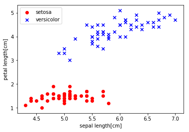
トレーニングデータの可視化コード
import pandas as pd
import matplotlib.pyplot as plt
import numpy as np

# irisデータを読み込み
df = pd.read_csv('https://archive.ics.uci.edu/ml/machine-learning-databases/iris/iris.data', header=None)
print(df.tail())

# 100行目までを抽出
y = df.iloc[0:100, 4].values
# 正解ラベルの変換
y = np.where(y == 'Iris-setosa', -1,1)
# 1行目と3行目を抽出する。
X = df.iloc[0:100, [0, 2]].values
# プロット
plt.scatter(X[:50,0], X[:50,1], color='red', marker='o', label='setosa')
plt.scatter(X[50:100,0], X[50:100,1], color='blue', marker='x', label='versicolor')
plt.xlabel('ガクの長さ[cm]')
plt.ylabel('花弁の長さ[cm]')
plt.legend(loc='upper left')
plt.show()
実行結果
       0    1    2    3               4
145  6.7  3.0  5.2  2.3  Iris-virginica
146  6.3  2.5  5.0  1.9  Iris-virginica
147  6.5  3.0  5.2  2.0  Iris-virginica
148  6.2  3.4  5.4  2.3  Iris-virginica
149  5.9  3.0  5.1  1.8  Iris-virginica
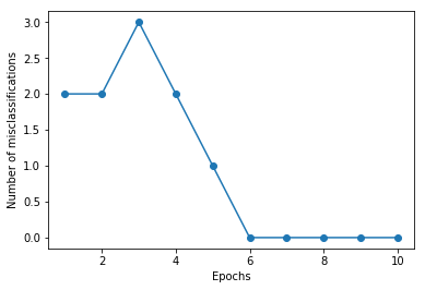
トレーニング
ppn = Perceptron(eta=0.1, n_iter=10)
ppn.fit(X, y)
plt.plot(range(1, len(ppn.errors_) + 1), ppn.errors_, marker='o')
plt.xlabel('Epochs')
plt.ylabel('Number of misclassifications')
plt.show()
実行結果
0 :  2
1 :  2
2 :  3
3 :  2
4 :  1
5 :  0
6 :  0
7 :  0
8 :  0
9 :  0
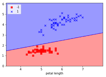
学習結果のプロット
from matplotlib.colors import ListedColormap

def plot_decision_regions(X, y, classifier, resolution = 0.02):
    # マーカーとカラーマップの準備
    markers = ('s', 'x', 'o', '^','v')
    colors = ('red', 'blue', 'lightgreen', 'grey', 'cyan')
    cmap = ListedColormap(colors[:len(np.unique(y))])

    #決定領域のプロット
    #X[:, 0]とやるとPandasのdataframeから各要素の0番目を取得できる
    x1_min, x1_max = X[:, 0].min() - 1, X[:, 0].max() + 1
    x2_min, x2_max = X[:, 1].min() - 1, X[:, 1].max() + 1
    #グリッドポイントの生成
    xx1, xx2 = np.meshgrid(np.arange(x1_min, x1_max, resolution), np.arange(x2_min, x2_max, resolution))
    #予測実行
    z = classifier.predict(np.array([xx1.ravel(), xx2.ravel()]).T)
    #予測結果を元のグリッドポイントのデータサイズに変換
    Z = z.reshape(xx1.shape)
    #グリッドポイントの等高線のプロット
    plt.contourf(xx1,xx2,Z,alpha=0.4,cmap=cmap)
    #軸の範囲の指定
    plt.xlim(xx1.min(), xx1.max())
    plt.ylim(xx2.min(), xx2.max())

    #クラスごとにサンプルをプロット
    for idx, cl in enumerate(np.unique(y)):
        plt.scatter(x=X[y == cl, 0], y=X[[y==cl, 1]], alpha=0.8, c=cmap(idx), marker=markers[idx],label=cl)

plot_decision_regions(X, y, classifier=ppn)
plt.xlabel('sepal length')
plt.xlabel('petal length')
plt.legend(loc='upper left')
plt.show()
実行結果

コメント