ADALINE

最近Python機械学習を読み進めているのですが、その学習メモです。
前回はこちら

パーセプトロンとの違いは、重みの更新方法

パーセプトロン：単位ステップ関数
ADALINE：線形活性化関数 $\phi(z)$

目的関数(Objective function) … 学習過程で最適化される関数。多くの場合は コスト関数 (cost function)

コスト関数

誤差平方和(Sum of Squared Error：SSE)
$$ J(w) = \frac{1}{2}\sum_i(y^{(i)}-\phi(z^{(i)}))^2 $$

利点

微分可能である
凸関数であるため勾配降下法(gradient descent)を用いてコスト関数を最小化する重みを見つけ出すことができる。

勾配降下法を使った重み更新

コスト関数$ J(w) $の勾配$ \nabla J(w) $に沿って1ステップ進む
$$ w := w + \Delta w $$
重みの変化である$ \Delta w $は、負の勾配に学習率$ \eta $を掛けたもの
$$ \Delta w = -\eta\nabla J(w) $$

勾配計算(偏微分係数)

$$ \begin{align} \frac{\delta J}{\delta w_j} &= \frac{\delta}{\delta w_j}\frac{1}{2}\sum_i(y^{(i)}-\phi(z^{(i)}))^2 \\
&= \frac{1}{2}\frac{\delta}{\delta w_j}\sum_i(y^{(i)}-\phi(z^{(i)}))^2 \\
&= \frac{1}{2}\sum_i2(y^{(i)}-\phi(z^{(i)}))\frac{\delta}{\delta w_j}(y^{(i)}-\phi(z^{(i)})) \\
&= \sum_i(y^{(i)}-\phi(z^{(i)}))\frac{\delta}{\delta w_j}\Bigl( y^{(i)}-\sum_k(w_kx_k^{(i)})\Bigr) \\
&= \sum_i(y^{(i)}-\phi(z^{(i)}))(-x_j^{(i)}) \\
&= -\sum_i(y^{(i)}-\phi(z^{(i)}))x_j^{(i)} \\
\end{align} $$

ADALINEの実装

class AdalineGD(object):
    """ADAptive LInear NEuron classifier.
 
    パラメータ
    ------------
    eta : float
        学習率 (0.0～1.0)
    n_iter : int
        繰り返し回数
 
    """
    def __init__(self, eta=0.01, n_iter=50):
        self.eta = eta
        self.n_iter = n_iter
 
    def fit(self, X, y):
        """ トレーニングデータの学習
 
        """
        self.w_ = np.zeros(1 + X.shape[1])
        self.cost_ = []
 
        for i in range(self.n_iter):
            net_input = self.net_input(X)
            output = self.activation(X)
            errors = (y - output)
            self.w_[1:] += self.eta * X.T.dot(errors)
            self.w_[0] += self.eta * errors.sum()
            cost = (errors**2).sum() / 2.0
            self.cost_.append(cost)
        return self
 
    def net_input(self, X):
        return np.dot(X, self.w_[1:]) + self.w_[0]
 
    def activation(self, X):
        return self.net_input(X)
 
    def predict(self, X):
        return np.where(self.activation(X) >= 0.0, 1, -1)

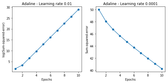
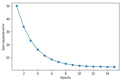
学習

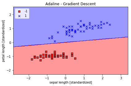
学習結果のプロット

from matplotlib.colors import ListedColormap
 
 
def plot_decision_regions(X, y, classifier, resolution=0.02):
 
    # setup marker generator and color map
    markers = ('s', 'x', 'o', '^', 'v')
    colors = ('red', 'blue', 'lightgreen', 'gray', 'cyan')
    cmap = ListedColormap(colors[:len(np.unique(y))])
 
    # plot the decision surface
    x1_min, x1_max = X[:, 0].min() - 1, X[:, 0].max() + 1
    x2_min, x2_max = X[:, 1].min() - 1, X[:, 1].max() + 1
    xx1, xx2 = np.meshgrid(np.arange(x1_min, x1_max, resolution),
                           np.arange(x2_min, x2_max, resolution))
    Z = classifier.predict(np.array([xx1.ravel(), xx2.ravel()]).T)
    Z = Z.reshape(xx1.shape)
    plt.contourf(xx1, xx2, Z, alpha=0.4, cmap=cmap)
    plt.xlim(xx1.min(), xx1.max())
    plt.ylim(xx2.min(), xx2.max())
 
    # plot class samples
    for idx, cl in enumerate(np.unique(y)):
        plt.scatter(x=X[y == cl, 0], y=X[y == cl, 1],
                    alpha=0.8, c=cmap(idx),
                    edgecolor='black',
                    marker=markers[idx], 
                    label=cl)