パーセプトロン – Python機械学習第三章学習メモ

最近Python機械学習を読み進めているのですが、その学習メモです。
前回はこちら

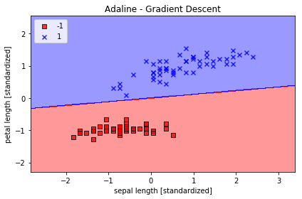
パーセプトロン

• irisデータセット用い、scikit-learnのパーセプトロンでトレーニングする
• 特徴量は萼片の長さと花弁の長さ

トレーニングデータの生成

from sklearn import datasets
import numpy as np
from sklearn.cross_validation import train_test_split
from sklearn.preprocessing import StandardScaler
from sklearn.linear_model import Perceptron
from sklearn.metrics import accuracy_score

# Irisデータセットをロード
iris = datasets.load_iris()
# 3,4列目の特徴量を抽出
X = iris.data[:, [2, 3]]
# クラスラベルを取得
y = iris.target
# print('Class labels:', np.unique(y))

# テストデータの分離
X_train, X_test, y_train, y_test = train_test_split(X, y, test_size=0.3, random_state=0)

# 特徴量のスケーリング
sc = StandardScaler()
# トレーニングデータの平均と標準偏差を計算
sc.fit(X_train)
# 平均と標準偏差を用いて標準化
X_train_std = sc.transform(X_train)
X_test_std = sc.transform(X_test)

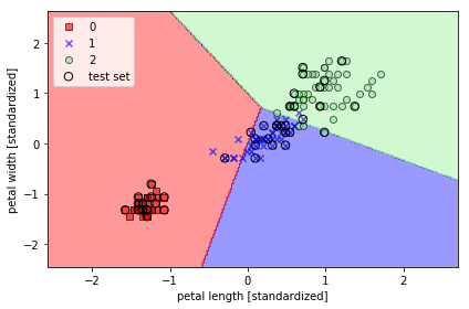
パーセプトロンを使用した学習

• scikit-learnのほとんどのアルゴリズムは多クラス分類をサポートしている。
• 多クラス分類には一対多(OvR)手法が使用される。

# パーセプトロンインスタンス生成
ppn = Perceptron(n_iter=40, eta0=0.1, random_state=0, shuffle=True)
# トレーニングデータをモデルに適合
ppn.fit(X_train_std, y_train)

y_pred = ppn.predict(X_test_std)
print('誤分類:%d' % (y_test != y_pred).sum())
print('正解率: %.2f' % accuracy_score(y_test, y_pred))

出力

誤分類:4
正解率: 0.91

学習結果のプロット

from matplotlib.colors import ListedColormap
import matplotlib.pyplot as plt
import warnings


def versiontuple(v):
    return tuple(map(int, (v.split("."))))


def plot_decision_regions(X, y, classifier, test_idx=None, resolution=0.02):

    # setup marker generator and color map
    markers = ('s', 'x', 'o', '^', 'v')
    colors = ('red', 'blue', 'lightgreen', 'gray', 'cyan')
    cmap = ListedColormap(colors[:len(np.unique(y))])

    # plot the decision surface
    x1_min, x1_max = X[:, 0].min() - 1, X[:, 0].max() + 1
    x2_min, x2_max = X[:, 1].min() - 1, X[:, 1].max() + 1
    xx1, xx2 = np.meshgrid(np.arange(x1_min, x1_max, resolution),
                           np.arange(x2_min, x2_max, resolution))
    Z = classifier.predict(np.array([xx1.ravel(), xx2.ravel()]).T)
    Z = Z.reshape(xx1.shape)
    plt.contourf(xx1, xx2, Z, alpha=0.4, cmap=cmap)
    plt.xlim(xx1.min(), xx1.max())
    plt.ylim(xx2.min(), xx2.max())

    for idx, cl in enumerate(np.unique(y)):
        plt.scatter(x=X[y == cl, 0],
                    y=X[y == cl, 1],
                    alpha=0.6,
                    c=cmap(idx),
                    edgecolor='black',
                    marker=markers[idx],
                    label=cl)

    # highlight test samples
    if test_idx:
        # plot all samples
        if not versiontuple(np.__version__) >= versiontuple('1.9.0'):
            X_test, y_test = X[list(test_idx), :], y[list(test_idx)]
            warnings.warn('Please update to NumPy 1.9.0 or newer')
        else:
            X_test, y_test = X[test_idx, :], y[test_idx]

        plt.scatter(X_test[:, 0],
                    X_test[:, 1],
                    c='',
                    alpha=1.0,
                    edgecolor='black',
                    linewidths=1,
                    marker='o',
                    s=55, label='test set')


X_combined_std = np.vstack((X_train_std, X_test_std))
y_combined = np.hstack((y_train, y_test))

plot_decision_regions(X=X_combined_std, y=y_combined,
                      classifier=ppn, test_idx=range(105, 150))
plt.xlabel('petal length [standardized]')
plt.ylabel('petal width [standardized]')
plt.legend(loc='upper left')

plt.tight_layout()
# plt.savefig('./figures/iris_perceptron_scikit.png', dpi=300)
plt.show()

実行結果