最近Python機械学習を読み進めているのですが、その学習メモです。
前回はこちら
SVM最適化の目的
マージンを最大化すること
- マージン:超平面(決定境界)と、この超平面に最も近いトレーニングサンプルの間の距離
- サポートベクトル:超平面に最も近いトレーニングサンプル
超平面
正の超平面
$$ w_0 + {\boldsymbol w^Tx_{pos}} = 1 $$
負の超平面
$$ w_0 + {\boldsymbol w^Tx_{neg}} = -1 $$
引き算して
$$ {\boldsymbol w^T(x_{pos} – x_{neg}}) = 2 $$
ここでベクトルの長さを以下のように定義する
$$ {\boldsymbol ||w||} = \sqrt{\sum_{j=1}^m w_j^2} $$
上2式から長さで割って標準化すると
$$ \frac{{\boldsymbol w^T(x_{pos} – x_{neg}})}{{\boldsymbol ||w||}} = \frac{2}{{\boldsymbol ||w||}} $$
左辺は正の超平面と負の超平面の距離 -> 最大化したいマージン
つまり、\( \frac{2}{{\boldsymbol ||w||}} \)の最大化がマージン最大化の問題である。
正のサンプルはすべて正の超平面の後ろに収まる。
$$ w_0 + {\boldsymbol w^Tx^{(i)}} \geq 1\; \; (y^{(i)} = 1)$$
負のサンプルはすべて負の超平面の側にある。
$$ w_0 + {\boldsymbol w^Tx^{(i)}} < -1\; \; (y^{(i)} = -1)$$
実際は、\( \frac{2}{{\boldsymbol ||w||}} \)の最大化ではなく逆数の二乗\( \frac{{\boldsymbol ||w||}^2}{2} \)の最小化の方が簡単。二次計画法により解くことができる。
スラック変数を使った非線形分離可能なケース
スラック変数:不等式制約を等式制約に変換するために導入する変数のこと
$$ {\boldsymbol w^Tx^{(i)}} \geq 1 – \xi^{(i)}\; (y^{(i)} = 1)$$
$$ {\boldsymbol w^Tx^{(i)}} < -1 + \xi^{(i)}\; (y^{(i)} = -1)$$
最小化すべき新しい対象は下記のとおり
$$ \frac{1}{2}{\boldsymbol ||w||^2} = C\biggl({\sum_{i}\xi^{(i)}}\biggr) $$
SVMを使ったIrisデータの分類
データの準備
from sklearn import datasets
import numpy as np
from sklearn.cross_validation import train_test_split
from sklearn.preprocessing import StandardScaler
from sklearn.linear_model import Perceptron
from sklearn.metrics import accuracy_score

# Irisデータセットをロード
iris = datasets.load_iris()
# 3,4列目の特徴量を抽出
X = iris.data[:, [2, 3]]
# クラスラベルを取得
y = iris.target
# print('Class labels:', np.unique(y))

# テストデータの分離
X_train, X_test, y_train, y_test = train_test_split(X, y, test_size=0.3, random_state=0)

# 特徴量のスケーリング
sc = StandardScaler()
# トレーニングデータの平均と標準偏差を計算
sc.fit(X_train)
# 平均と標準偏差を用いて標準化
X_train_std = sc.transform(X_train)
X_test_std = sc.transform(X_test)

from sklearn.preprocessing import StandardScaler
sc = StandardScaler()
sc.fit(X_train)
X_train_std = sc.transform(X_train)
X_test_std = sc.transform(X_test)
X_combined_std = np.vstack((X_train_std, X_test_std))
y_combined = np.hstack((y_train, y_test))
プロット関数
from matplotlib.colors import ListedColormap
import matplotlib.pyplot as plt
import warnings

def versiontuple(v):
    return tuple(map(int, (v.split("."))))


def plot_decision_regions(X, y, classifier, test_idx=None, resolution=0.02):

    # setup marker generator and color map
    markers = ('s', 'x', 'o', '^', 'v')
    colors = ('red', 'blue', 'lightgreen', 'gray', 'cyan')
    cmap = ListedColormap(colors[:len(np.unique(y))])

    # plot the decision surface
    x1_min, x1_max = X[:, 0].min() - 1, X[:, 0].max() + 1
    x2_min, x2_max = X[:, 1].min() - 1, X[:, 1].max() + 1
    xx1, xx2 = np.meshgrid(np.arange(x1_min, x1_max, resolution),
                           np.arange(x2_min, x2_max, resolution))
    Z = classifier.predict(np.array([xx1.ravel(), xx2.ravel()]).T)
    Z = Z.reshape(xx1.shape)
    plt.contourf(xx1, xx2, Z, alpha=0.4, cmap=cmap)
    plt.xlim(xx1.min(), xx1.max())
    plt.ylim(xx2.min(), xx2.max())

    for idx, cl in enumerate(np.unique(y)):
        plt.scatter(x=X[y == cl, 0],
                    y=X[y == cl, 1],
                    alpha=0.6,
                    c=cmap(idx),
                    edgecolor='black',
                    marker=markers[idx],
                    label=cl)

    # highlight test samples
    if test_idx:
        # plot all samples
        if not versiontuple(np.__version__) >= versiontuple('1.9.0'):
            X_test, y_test = X[list(test_idx), :], y[list(test_idx)]
            warnings.warn('Please update to NumPy 1.9.0 or newer')
        else:
            X_test, y_test = X[test_idx, :], y[test_idx]

        plt.scatter(X_test[:, 0],
                    X_test[:, 1],
                    c='',
                    alpha=1.0,
                    edgecolor='black',
                    linewidths=1,
                    marker='o',
                    s=55, label='test set')
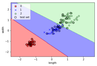
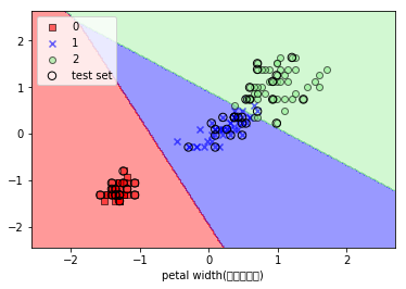
SVMで分類・表示
from sklearn.svm import SVC
svm = SVC(kernel='linear', C=1.0, random_state=0)
svm.fit(X_train_std, y_train)
plot_decision_regions(X_combined_std, y_combined, classifier=svm, test_idx=range(105,150))
plt.xlabel('length')
plt.ylabel('width')
plt.legend(loc='upper left')
plt.show()
実行結果
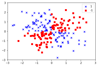
カーネルSVMを使って非線形問題の解を求める
XORデータセットを作成する
np.random.seed(0)
X_xor = np.random.randn(200, 2)
y_xor = np.logical_xor(X_xor[:, 0] > 0, X_xor[:, 1] > 0)
y_xor = np.where(y_xor, 1, -1)
plt.scatter(X_xor[y_xor==1, 0], X_xor[y_xor==1, 1], c='b', marker='x', label='1')
plt.scatter(X_xor[y_xor==-1, 0], X_xor[y_xor==-1, 1], c='r', marker='s', label='-1')
plt.xlim([-3, 3])
plt.ylim([-3, 3])
plt.legend(loc='best')
plt.show()
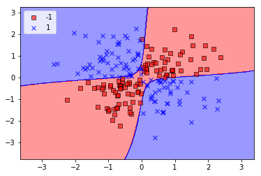
カーネルトリックを使って分離超平面を高次元空間で特定する
非線形の解は射影関数\( \phi(\cdot) \)を使ってトレーニングセットをより高い次元の特徴空間に移すことで可能となる。しかし、計算コストが高いのでカーネル関数を定義する。
$$ k({\boldsymbol x^{(i)}},{\boldsymbol x^{(j)}}) = \phi({\boldsymbol x^{(i)}})^T\phi({\boldsymbol x^{(j)}}) $$
- カーネル:2つのサンプル間の「類似性を表す関数」。
- 類似度は1(全く同じ)から0(全く異なる)の間。
最も広く利用されているカーネルは動径基底関数カーネル(Radial Basis Function kernel:RBF)。ガウスカーネルとも。
$$ k({\boldsymbol x^{(i)}},{\boldsymbol x^{(j)}}) = \exp\biggl(-\frac{{||\boldsymbol x^{(i)}} – {\boldsymbol x^{(j)}}||^2}{2\sigma^2}\biggr) $$
簡略化版
$$ k({\boldsymbol x^{(i)}},{\boldsymbol x^{(j)}}) = \exp\bigl(-\gamma{||\boldsymbol x^{(i)}} – {\boldsymbol x^{(j)}}||^2\bigr) $$
\( \gamma = \frac{1}{2\sigma^2} \)が最適化されるハイパーパラメータ。
# 上のコードのkernel='linear'を'rbf'に置き換える
svm = SVC(kernel='rbf', random_state=0, gamma=0.1, C=10.0)
svm.fit(X_xor, y_xor)
plot_decision_regions(X_xor,y_xor, classifier=svm)
plt.legend(loc='upper left')
plt.show()
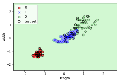
Irisデータに対してgammaを変えて適用してみる
gammaを色々変えると面白い。大きくすればするほどトレーニングデータにフィットするが、過学習になる。
svm = SVC(kernel='rbf', C=1.0, random_state=0, gamma=100)
svm.fit(X_train_std, y_train)
plot_decision_regions(X_combined_std, y_combined, classifier=svm, test_idx=range(105,150))
plt.xlabel('length')
plt.ylabel('width')
plt.legend(loc='upper left')
plt.show()

コメント
はじめまして。
最近Pythonによる機械学習を始めた大学生です。
独学なのでブログを参考にさせていただいております。
もし可能であれば4章以降の学習メモもブログにあげていただけると非常に助かります。
よろしくお願いします。
コメントありがとうございます!
ちょっと更新停滞気味でしたがまた再開します(`・ω・´)